
This post introduces how to use BitSwan Jupyter Automations to create your first automation using a WebForm source. You’ll learn how to set up a simple automation pipeline, define a web form, and handle the data submitted through it.
We will follow an automation that is present in our examples: StocksCalculator. Feel free to experiment yourself, but this following tutorial will go to detail how each component works.
This tutorial will give you an example of an automation where you can select a date and the pipeline will display a graph of the several stocks and their performance at that day!
The resulting automation will look like this: automation
Jupyter Automation
If you have a BitSwan workspace with the VS Code editor and the BitSwan extension installed, you’re ready to get started. Below is an example automation script. We’ll go through it cell by cell and explain each part of the pipeline.
1. Import Required Modules
from bspump.jupyter import *
from bspump.http.web.server import *
import requests
import pandas as pd
from datetime import datetime, timedelta
import matplotlib
import time
import io
from datetime import date
import base64
The first cell as usual imports the necessary modules.
bspump.jupytermodule is used to run and handle the automation in the jupyter notebook.- The
bspump.http.web.servermodule is used to create a web server that will serve the web form.
The rest of libraries are the usual libraries you might know using python.
pandasis for data processingrequestsfor sending requests via http/httpsdatetimeworking with dates etc.
2. Define an Initial Event (For Dev Execution)
event = {
    "form": {
        "Year": 2025,
        "Month": 6,
        "Day": 5
    }
}
This optional cell defines an event dictionary, alowing us to execute all cells during development to test the automation.
3. Define the Automation Pipeline
auto_pipeline(
    source=lambda app, pipeline: WebFormSource(app, pipeline, route="/",
    form_intro="""<p> Select date range and click submit to see a visualization""",
    fields=[
        IntField("Day",default=20),
        IntField("Month",default=2),
        IntField("Year",default=2025),
    ]),
    sink=lambda app, pipeline: WebSink(app, pipeline)
)
This is the core of the automation. We use auto_pipeline to define our pipeline with minimal boilerplate:
- Source:
WebFormSourcerenders a form at the root path (/) with a set of fields. - Sink:
WebSinkhandles the final processed output of the automation. and displays it on the web page. In this case it will render an jpeg of a graph.
The form can include:
- Text fields (some with defaults or hidden)
- An integer input
- A dropdown (choice field)
- A checkbox
In this case we are using three fields for day, month and year.
You can mix and match different sources and sinks to create your desired automation.
List of available sources and sinks can be found in the BitSwan library. List includes: Kafka, WebFormSource, Slack, MongoDB, PostgreSQL, GoogleDrive and many more… In case you would like to see another examples of working pipelines, you can check the BitSwan examples
5. helper output formatting
You can copy the following functions. They define how the automation’s output is displayed to the user using HTML and CSS styling to ensure a clean and user-friendly presentation.
def output_layout(parsed_date,top_stock_name,top_stock_change,img_data) -> str:
    html = f"""
    <!DOCTYPE html>
    <html>
    <head>
        <title>Stock Performance</title>
        <style>
            body {{
                font-family: Arial, sans-serif;
                text-align: center;
                background-color: #f5f5f5;
                padding: 40px;
            }}
            h1 {{
                color: #333;
                margin-bottom: 20px;
            }}
            img {{
                border: 1px solid #ccc;
                max-width: 90%;
                height: auto;
                box-shadow: 0 0 10px rgba(0,0,0,0.1);
            }}
            button {{
                background-color: #0275d8;
                color: white;
                border: none;
                padding: 10px 20px;
                font-size: 16px;
                border-radius: 5px;
                cursor: pointer;
            }}
            button:hover {{
                background-color: #025aa5;
            }}
        </style>
    </head>
    <body>
        <h1>📈 Top Stock on {parsed_date}: {top_stock_name} (change {top_stock_change:.2f}%)</h1>
        <img src="data:image/jpeg;base64,{base64.b64encode(img_data.getvalue()).decode()}" alt="Stock Performance">
        <button onclick="window.history.back()">🔙 Go Back</button>
    </body>
    </html>
    """
    return html


def output_no_data_found() -> str:
    html = """
    <!DOCTYPE html>
    <html>
    <head>
       <title>No Data Found</title>
        <style>
            body {
                font-family: Arial, sans-serif;
                text-align: center;
                background-color: #f5f5f5;
                padding: 40px;
            }
            h1 {
                color: #d9534f;
                margin-bottom: 20px;
            }
            p {
                color: #555;
                font-size: 18px;
                margin-bottom: 30px;
            }
            button {
                background-color: #0275d8;
                color: white;
                border: none;
                padding: 10px 20px;
                font-size: 16px;
                border-radius: 5px;
                cursor: pointer;
            }
            button:hover {
                background-color: #025aa5;
            }
        </style>
    </head>
    <body>
        <h1>⚠️ No Stock Data Found</h1>
        <p>Markets might be closed, try a different date.</p>
        <button onclick="window.history.back()">🔙 Go Back</button>
    </body>
    </html>
    """
    return html
6. Handle pipeline logic, Global variables and Input Handling
# Global variables
STOCKS = ["AAPL", "MSFT", "GOOGL", "AMZN", "TSLA", "NVDA", "META", "JPM", "NFLX", "AMD"]

HEADERS = {
        "User-Agent": "Mozilla/5.0 (Windows NT 10.0; Win64; x64)"
        }

# Input processing
form = event["form"]
parsed_date_str = date(form["Year"], form["Month"], form["Day"]).strftime("%Y-%m-%d")
parsed_date = datetime.strptime(parsed_date_str, "%Y-%m-%d")
day_before = parsed_date - timedelta(days=1)
day_after = parsed_date + timedelta(days=1)
Cell below the automation_pipeline definition are executed when the pipeline is triggered.
In this case:
- Once the form is sumitted,
WebFormSourcecreates an event. - The
eventobject includes the submittedformdata.
We also define global variables that are used later on.
7. Cell for fetching Yahoo data and performing calculations
# Initialize change tracking
changes = {}

# Iterate over each ticker and fetch data
for ticker in STOCKS:
    # Convert datetime to UNIX timestamps
    start_ts = int(time.mktime(day_before.timetuple()))
    end_ts = int(time.mktime(day_after.timetuple()))

    # Prepare API request
    url = f"https://query1.finance.yahoo.com/v8/finance/chart/{ticker}"
    params = {
        "period1": start_ts,
        "period2": end_ts,
        "interval": "1d"
    }

    try:
        response = requests.get(url, params=params, headers=HEADERS)
        data = response.json()

        result = data["chart"]["result"][0]
        timestamps = result["timestamp"]
        closes = result["indicators"]["quote"][0]["close"]

        # Convert timestamps to readable dates
        dates = [datetime.fromtimestamp(ts).strftime('%Y-%m-%d') for ts in timestamps]
        series = pd.Series(closes, index=dates)

        # Compute percent change if both dates exist in the series
        if parsed_date_str in series and day_before.strftime("%Y-%m-%d") in series:
            previous_close = series[day_before.strftime("%Y-%m-%d")]
            current_close = series[parsed_date_str]
            if previous_close and current_close:
                percent_change = ((current_close - previous_close) / previous_close) * 100
                changes[ticker] = percent_change

    except Exception as e:
        print(f"Error fetching data for {ticker}: {e}")
In this cell, we process the input data and perform most of the logic needed to obtain results that can then be plotted.
8. Cell for plotting the Stock changes.
# install matplotlib if you experience error with the plot while executing the cells in during dev
# %pip install matplotlib

# Prepare output if data is available
if changes:
    df = pd.DataFrame(list(changes.items()), columns=["Ticker", "Change (%)"])
    df.sort_values("Change (%)", ascending=False, inplace=True)

    # Plotting
    ax = df.plot.bar(
        x="Ticker",
        y="Change (%)",
        title=f"Stock Change (%) on {parsed_date_str}",
        xlabel="Ticker",
        ylabel="Change (%)",
        grid=True,
        figsize=(10, 7)
    )

    # Save plot to buffer
    buf = io.BytesIO()
    ax.figure.savefig(buf, format="jpeg")
    img_data = buf
This cell defines the DataFrame and the plot layout. If you created a mock event earlier, you can test the plot and should see something like this:
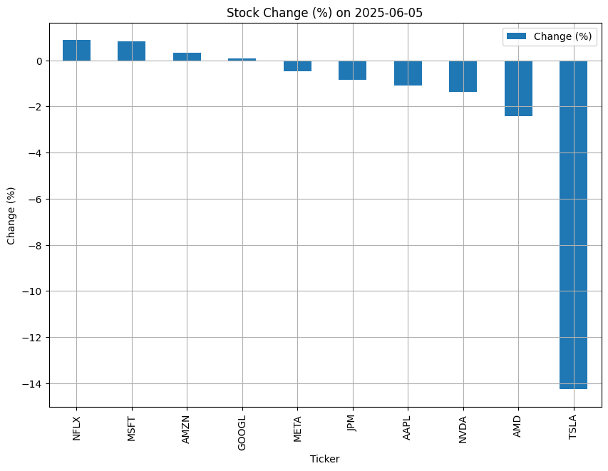
As you can see, on July 5th, 2025, Tesla stock experienced a sharp downward spike.
8. Prepare the output for the WebSink
if changes:
    # Get top stock info
    top_stock = max(changes, key=changes.get)
    top_stock_name = top_stock
    top_stock_change = changes[top_stock]

    # Build and set response
    response = output_layout(
        parsed_date=parsed_date_str,
        top_stock_name=top_stock_name,
        top_stock_change=top_stock_change,
        img_data=img_data
    )

    event["response"] = response
    event["content_type"] = "text/html"

else:
    event["response"] = output_no_data_found()
    event["content_type"] = "text/html"
We consturct a new response field in the event using the helper styling functions. Note that we set the content_type to text/html, so the HTML is rendered properly.
Since this is the last cell of the automation and it contains the event object, it will be automatically sent as input to the WebSink.
It’s important to note that your automation can include any functionality you need. The WebFormSource simply acts as a trigger - what you do with the Jupyter cells and the event data is entirely up to you.
Wow! You’ve just created your first automation using a WebForm source.
6. Run the automation
You can execute the cells to check whether the data loads and the plot renders correctly without errors. Once you’re satisfied, you can deploy the automation using the BitSwan extension.
If you’re unable to deploy the automation yourself, you can try this live version: automation
Conclusion
In this guide, we walked through the process of creating a WebForm-based automation using BitSwan Jupyter Automations. You learned how to:
Import and set up required modules
Define a form-based source
Process and structure incoming form data
Output the final result via a sink
This example is a great starting point. From here, you can expand your automations with custom logic, additional sources and sinks, and other powerful BitSwan capabilities.
If you have any questions or need assistance, feel free to reach out — we’re here to help!
Happy automating! 🚀